初始化 这次编程作业对比了三种不同的初始化方法的不同,三种方法分别是“零初始化”、“随机初始化”、“He 初始化”。
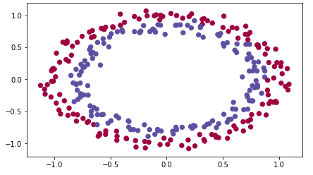
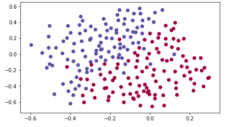
这是所用的数据,我们要将红点和蓝点分类:
零初始化 也就是将参数 w 和 b 全都初始化为 0,代码如下:
1
2
3
4
5
6
7
8
9
def initialize_parameters_zeros (layers_dims) : parameters = {} L = len(layers_dims) for l in range(1 , L): parameters['W' + str(l)] = np.zeros((layers_dims[l],layers_dims[l-1 ])) parameters['b' + str(l)] = np.zeros((layers_dims[l],1 )) return parameters
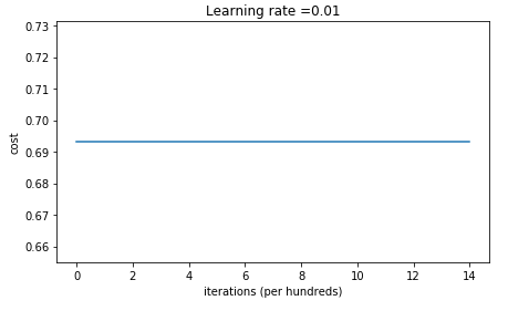
最后的代价函数随迭代次数的变化如下:
训练集的精确度为 0.5,测试集的精确度为 0.5
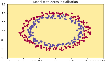
分类结果如下:
我们可以发现将所有参数初始化为零无法分类任何数据,因为无法打破对称性,这意味着每层的每个神经元都在学习一样的东西。
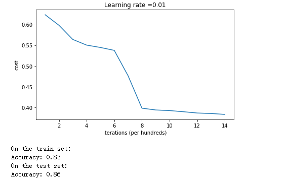
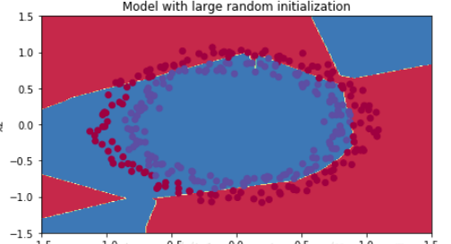
随机初始化(为很大的值) 将权重矩阵随机地初始化为很大的值(×10),偏差向量继续初始化为零,代码如下:
1
2
3
4
5
6
7
8
9
10
def initialize_parameters_random (layers_dims) : parameters = {} L = len(layers_dims) for l in range(1 , L): parameters['W' + str(l)] = np.random.randn(layers_dims[l],layers_dims[l-1 ])*10 parameters['b' + str(l)] = np.zeros((layers_dims[l],1 )) return parameters
代价函数的变化如下:
训练集精确度为 0.83,测试集为 0.86
分类的结果为:
分析:
代价函数开始的值很高,是因为用很大的随机值初始化权重会使得最后的激活(sigmoid)输出值 $a^{[L]}$ 非常接近 0 或者 1,代价函数公式为$J = - \frac{1}{m} \sum\limits_{i = 0}^{m} \large{(} \small y^{(i)}\log\left(a^{[L] (i)}\right) + (1-y^{(i)})\log\left(1- a^{[L] (i)}\right) \large{)} \small$ ,当 $a^{[ L ] ( i )} \approx 0$ 时,$log(a^{[ L ] ( i )})= log( 0 ) \rightarrow$ 无穷大
不好的初始化可能导致梯度消失/爆炸,这会减慢优化算法的速度
如果训练上面的的网络更长时间,可以得到更好的结果,但是用大随机值初始化会减慢优化的速度
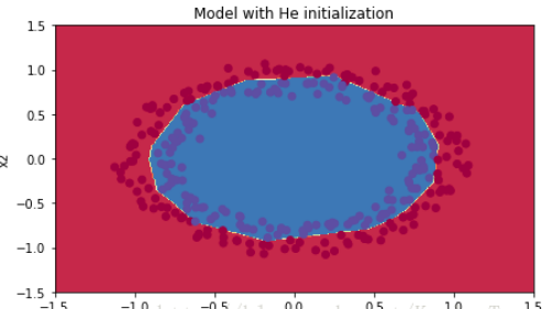
He初始化 这是用某个人名命名的初始化,与上面的随机初始化相似,只是在末尾不是乘以 10 而是 $\sqrt{\frac{2}{n^{[l-1]}}}$ ,这个推荐用来初始化包含 relu 激活函数的层,代码如下:
1
2
3
4
5
6
7
8
9
10
def initialize_parameters_he (layers_dims) : parameters = {} L = len(layers_dims) - 1 for l in range(1 , L + 1 ): parameters['W' + str(l)] = np.random.randn(layers_dims[l],layers_dims[l-1 ])*np.sqrt(2 /layers_dims[l-1 ]) parameters['b' + str(l)] = np.zeros((layers_dims[l],1 )) return parameters
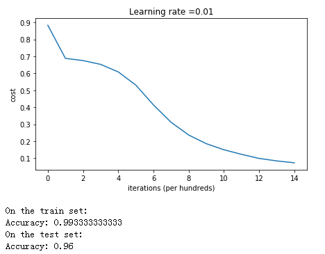
代价函数图像如下:
训练集上的精确度达到了 0.99,测试集上的精确度达到了 0.96
分类的结果如下:
分析:我们可以看到 He 初始化在很少的迭代次数上就将蓝点和红点分类得很好
结论
不同的初始化有不同的结果
随机初始化用来打破权重对称确保不同的隐藏层能学习到不同的东西
不要把任何值初始化得太大
对于有 relu 激活函数的网络 He 初始化非常有效
正则化 本次编程作业将会学到如何在深度学习模型中运用正则化。
包的引入 1 2 3 4 5 6 7 8 9 10 11 12 13 14 import numpy as npimport matplotlib.pyplot as pltfrom reg_utils import sigmoid, relu, plot_decision_boundary, initialize_parameters, load_2D_dataset, predict_decfrom reg_utils import compute_cost, predict, forward_propagation, backward_propagation, update_parametersimport sklearnimport sklearn.datasetsimport scipy.iofrom testCases import *%matplotlib inline plt.rcParams['figure.figsize' ] = (7.0 , 4.0 ) plt.rcParams['image.interpolation' ] = 'nearest' plt.rcParams['image.cmap' ] = 'gray'
数据集 1 train_X, train_Y, test_X, test_Y = load_2D_dataset()
非正则化模型 将正则化系数 lambd 设为 0,将 keep_prob 设为 1,模型如下:
1 2 3 4 5 6 7 8 9 10 11 12 13 14 15 16 17 18 19 20 21 22 23 24 25 26 27 28 29 30 31 32 33 34 35 36 37 38 39 40 41 42 43 44 45 46 47 48 49 50 51 52 53 54 55 56 57 58 59 60 61 62 63 64 65 66 def model (X, Y, learning_rate = 0.3 , num_iterations = 30000 , print_cost = True, lambd = 0 , keep_prob = 1 ) : """ 实现一个三层的神经网络: 线性->RELU->线性->RELU->线性->SIGMOID. Arguments: X -- input data, of shape (input size, number of examples) Y -- true "label" vector (1 for blue dot / 0 for red dot), of shape (output size, number of examples) learning_rate -- learning rate of the optimization num_iterations -- number of iterations of the optimization loop print_cost -- If True, print the cost every 10000 iterations lambd -- regularization hyperparameter, scalar keep_prob - probability of keeping a neuron active during drop-out, scalar. Returns: parameters -- parameters learned by the model. They can then be used to predict. """ grads = {} costs = [] m = X.shape[1 ] layers_dims = [X.shape[0 ], 20 , 3 , 1 ] parameters = initialize_parameters(layers_dims) for i in range(0 , num_iterations): if keep_prob == 1 : a3, cache = forward_propagation(X, parameters) elif keep_prob < 1 : a3, cache = forward_propagation_with_dropout(X, parameters, keep_prob) if lambd == 0 : cost = compute_cost(a3, Y) else : cost = compute_cost_with_regularization(a3, Y, parameters, lambd) assert (lambd==0 or keep_prob==1 ) if lambd == 0 and keep_prob == 1 : grads = backward_propagation(X, Y, cache) elif lambd != 0 : grads = backward_propagation_with_regularization(X, Y, cache, lambd) elif keep_prob < 1 : grads = backward_propagation_with_dropout(X, Y, cache, keep_prob) parameters = update_parameters(parameters, grads, learning_rate) if print_cost and i % 10000 == 0 : print("Cost after iteration {}: {}" .format(i, cost)) if print_cost and i % 1000 == 0 : costs.append(cost) plt.plot(costs) plt.ylabel('cost' ) plt.xlabel('iterations (x1,000)' ) plt.title("Learning rate =" + str(learning_rate)) plt.show() return parameters
我们先不使用正则化试试:
1
2
3
4
5
parameters = model(train_X, train_Y) print ("On the training set:" )predictions_train = predict(train_X, train_Y, parameters) print ("On the test set:" )predictions_test = predict(test_X, test_Y, parameters)
结果是:
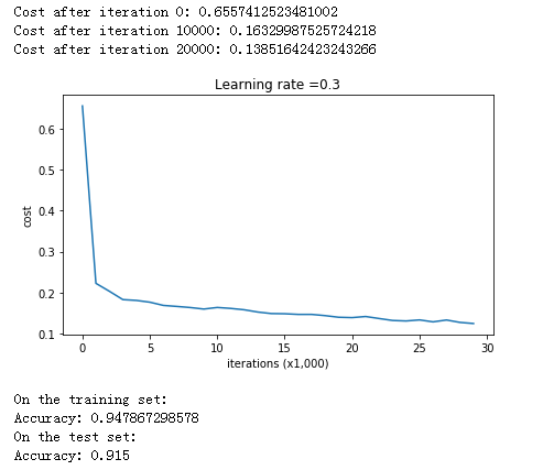
在测试集上的精确度为 0.91,而在训练集上的有 0.95,打印出分类图像看看:
很明显,分类器将一些训练集中的噪声学习进去了,发生了过拟合,接下来用正则化试试。
L2 正则化 实现 代价函数为:
L2 正则化是在原本代价函数的基础上加上一个正则化项:
计算带有正则化项的代价函数:
1
2
3
4
5
6
7
8
9
10
11
12
13
14
15
16
17
18
19
20
21
22
23
24
def compute_cost_with_regularization (A3, Y, parameters, lambd) : """ 计算带有 L2 正则化项的代价函数 Arguments: A3 -- post-activation, output of forward propagation, of shape (output size, number of examples) Y -- "true" labels vector, of shape (output size, number of examples) parameters -- python dictionary containing parameters of the model Returns: cost - value of the regularized loss function (formula (2)) """ m = Y.shape[1 ] W1 = parameters["W1" ] W2 = parameters["W2" ] W3 = parameters["W3" ] cross_entropy_cost = compute_cost(A3, Y) L2_regularization_cost = (lambd/(2 *m))*(np.sum(np.square(W1))+np.sum(np.square(W2))+np.sum(np.square(W3))) cost = cross_entropy_cost + L2_regularization_cost return cost
由于代价函数变了,所以反向传播计算某个参数的梯度也要加上正则化项对它的梯度:$\frac{d}{dW} ( \frac{1}{2}\frac{\lambda}{m} W^2) = \frac{\lambda}{m} W$
1
2
3
4
5
6
7
8
9
10
11
12
13
14
15
16
17
18
19
20
21
22
23
24
25
26
27
28
29
30
31
32
33
34
35
36
37
38
39
def backward_propagation_with_regularization (X, Y, cache, lambd) : """ 用带了正则化项的代价函数计算反向传播 Arguments: X -- input dataset, of shape (input size, number of examples) Y -- "true" labels vector, of shape (output size, number of examples) cache -- 前向传播缓存 lambd -- regularization hyperparameter, scalar Returns: gradients -- A dictionary with the gradients with respect to each parameter, activation and pre-activation variables """ m = X.shape[1 ] (Z1, A1, W1, b1, Z2, A2, W2, b2, Z3, A3, W3, b3) = cache dZ3 = A3 - Y dW3 = 1. /m * np.dot(dZ3, A2.T) + (lambd / m * W3) db3 = 1. /m * np.sum(dZ3, axis=1 , keepdims = True ) dA2 = np.dot(W3.T, dZ3) dZ2 = np.multiply(dA2, np.int64(A2 > 0 )) dW2 = 1. /m * np.dot(dZ2, A1.T) + (lambd / m * W2) db2 = 1. /m * np.sum(dZ2, axis=1 , keepdims = True ) dA1 = np.dot(W2.T, dZ2) dZ1 = np.multiply(dA1, np.int64(A1 > 0 )) dW1 = 1. /m * np.dot(dZ1, X.T) + (lambd / m * W1) db1 = 1. /m * np.sum(dZ1, axis=1 , keepdims = True ) gradients = {"dZ3" : dZ3, "dW3" : dW3, "db3" : db3,"dA2" : dA2, "dZ2" : dZ2, "dW2" : dW2, "db2" : db2, "dA1" : dA1, "dZ1" : dZ1, "dW1" : dW1, "db1" : db1} return gradients
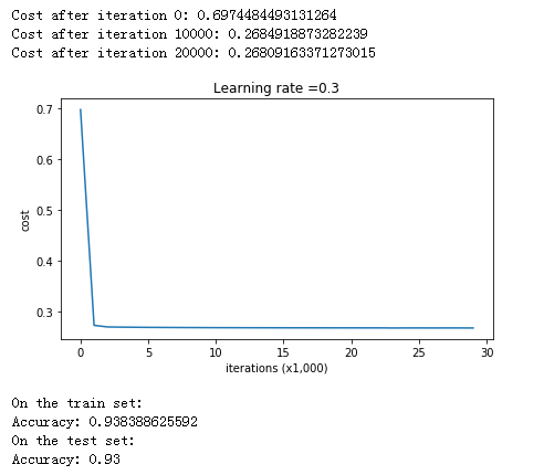
现在将正则化系数 lambd 设为 0.7 看看效果:
1
2
3
4
5
parameters = model(train_X, train_Y, lambd = 0.7 ) print ("On the train set:" )predictions_train = predict(train_X, train_Y, parameters) print ("On the test set:" )predictions_test = predict(test_X, test_Y, parameters)
结果如下:
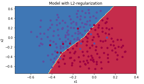
测试集精确度提高到了 0.93,打印分类图像:
1 2 3 4 5 plt.title("Model with L2-regularization" ) axes = plt.gca() axes.set_xlim([-0.75 ,0.40 ]) axes.set_ylim([-0.75 ,0.65 ]) plot_decision_boundary(lambda x: predict_dec(parameters, x.T), train_X, train_Y)
可以看到噪点已经没有被学习进去。
分析
正则化参数 $\lambda$ 是一个可以在开发集上调整的超参数
L2 正则化让分类的边界更加平滑,但是如果正则化参数太大,则很可能导致“过平滑”,即变成一根直线,造成很大的偏差
L2 正则化的原理 L2 正则化依赖于一个假设,即权重更小的模型比权重更大的模型更简单,所以,通过在代价函数里惩罚 权重的平方值,驱使所有的权重值变得更小,因为如果你有高权重值,那么代价函数就会变得非常大!这生成了一个更加平滑的模型,在模型中输出改变得比输入更慢。
总结
代价函数计算:正则化项应该加进代价函数中
反向传播:在代价函数对权重的梯度中应该加入正则化项对其的梯度
权重最后被驱使变得更小:权重衰减
dropout 正则化 dropout 技术的原理 dropout 正则化在每次迭代中丢弃一些结点,也就是将这些结点的激活值变成零,每个结点被保留的概率是 keep_prob,被丢弃的结点在整个这次迭代过程中都不会出现。
当你丢弃某些神经元时,实际上改变了模型的结构,每一次迭代,你都在训练不同的模型,而这些模型是原有模型的子集。使用 dropout 让神经元们对某个特定的神经元的激活不再那么敏感,因为它随时可能会被丢弃。
实现 首先在前向传播中实现 dropout,假设是第 l 层,一共有如下四步:
代码如下:
1
2
3
4
5
6
7
8
9
10
11
12
13
14
15
16
17
18
19
20
21
22
23
24
25
26
27
28
29
30
31
32
33
34
35
36
37
38
39
40
41
42
43
44
45
46
47
48
49
50
51
52
53
def forward_propagation_with_dropout (X, parameters, keep_prob = 0.5 ) : """ 实现带 dropout 的前向传播: LINEAR -> RELU + DROPOUT -> LINEAR -> RELU + DROPOUT -> LINEAR -> SIGMOID. Arguments: X -- input dataset, of shape (2, number of examples) parameters -- python dictionary containing your parameters "W1", "b1", "W2", "b2", "W3", "b3": W1 -- weight matrix of shape (20, 2) b1 -- bias vector of shape (20, 1) W2 -- weight matrix of shape (3, 20) b2 -- bias vector of shape (3, 1) W3 -- weight matrix of shape (1, 3) b3 -- bias vector of shape (1, 1) keep_prob - probability of keeping a neuron active during drop-out, scalar Returns: A3 -- last activation value, output of the forward propagation, of shape (1,1) cache -- tuple, information stored for computing the backward propagation """ W1 = parameters["W1" ] b1 = parameters["b1" ] W2 = parameters["W2" ] b2 = parameters["b2" ] W3 = parameters["W3" ] b3 = parameters["b3" ] Z1 = np.dot(W1, X) + b1 A1 = relu(Z1) D1 = np.random.rand(A1.shape[0 ], A1.shape[1 ]) D1 = D1 < keep_prob A1 = A1 * D1 A1 = A1 / keep_prob Z2 = np.dot(W2, A1) + b2 A2 = relu(Z2) D2 = np.random.rand(A2.shape[0 ],A2.shape[1 ]) D2 = D2 < keep_prob A2 = A2 * D2 A2 = A2 / keep_prob Z3 = np.dot(W3, A2) + b3 A3 = sigmoid(Z3) cache = (Z1, D1, A1, W1, b1, Z2, D2, A2, W2, b2, Z3, A3, W3, b3) return A3, cache
然后我们在反向传播中使用 dropout,一共两步:
将每层的筛选矩阵 D[i] 从缓存中取出,将 dA[i] 也乘上筛选矩阵,因为一个结点被丢弃后该结点的梯度值也归零
由于 A[i] 除以了 keep_prob,它对应的 dA[i] 也应该除以 keep_prob 来进行补偿
反向传播函数代码如下:
1
2
3
4
5
6
7
8
9
10
11
12
13
14
15
16
17
18
19
20
21
22
23
24
25
26
27
28
29
30
31
32
33
34
35
36
37
38
39
40
41
42
43
44
def backward_propagation_with_dropout (X, Y, cache, keep_prob) : """ 实现加了 dropout 的反向传播 Arguments: X -- input dataset, of shape (2, number of examples) Y -- "true" labels vector, of shape (output size, number of examples) cache -- cache output from forward_propagation_with_dropout() keep_prob - probability of keeping a neuron active during drop-out, scalar Returns: gradients -- A dictionary with the gradients with respect to each parameter, activation and pre-activation variables """ m = X.shape[1 ] (Z1, D1, A1, W1, b1, Z2, D2, A2, W2, b2, Z3, A3, W3, b3) = cache dZ3 = A3 - Y dW3 = 1. /m * np.dot(dZ3, A2.T) db3 = 1. /m * np.sum(dZ3, axis=1 , keepdims = True ) dA2 = np.dot(W3.T, dZ3) dA2 = dA2 * D2 dA2 = dA2 / keep_prob dZ2 = np.multiply(dA2, np.int64(A2 > 0 )) dW2 = 1. /m * np.dot(dZ2, A1.T) db2 = 1. /m * np.sum(dZ2, axis=1 , keepdims = True ) dA1 = np.dot(W2.T, dZ2) dA1 = dA1 * D1 dA1 = dA1 / keep_prob dZ1 = np.multiply(dA1, np.int64(A1 > 0 )) dW1 = 1. /m * np.dot(dZ1, X.T) db1 = 1. /m * np.sum(dZ1, axis=1 , keepdims = True ) gradients = {"dZ3" : dZ3, "dW3" : dW3, "db3" : db3,"dA2" : dA2, "dZ2" : dZ2, "dW2" : dW2, "db2" : db2, "dA1" : dA1, "dZ1" : dZ1, "dW1" : dW1, "db1" : db1} return gradients
现在运行使用了 dropout 的模式试试:
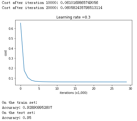
1
2
3
4
5
6
parameters = model(train_X, train_Y, keep_prob = 0.86 , learning_rate = 0.3 ) print ("On the train set:" )predictions_train = predict(train_X, train_Y, parameters) print ("On the test set:" )predictions_test = predict(test_X, test_Y, parameters)
注意:不要在测试过程中使用 dropout!!
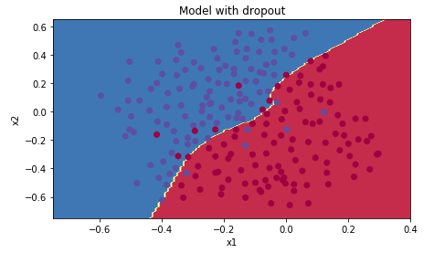
测试集精度提高到了 0.95!画图看看分类的结果:
1 2 3 4 5 plt.title("Model with dropout" ) axes = plt.gca() axes.set_xlim([-0.75 ,0.40 ]) axes.set_ylim([-0.75 ,0.65 ]) plot_decision_boundary(lambda x: predict_dec(parameters, x.T), train_X, train_Y)
总结
dropout 是一门正则化技术
只在训练时使用 dropout,不要在测试时使用
在前向和反向传播中都要同时使用 dropout
在前向传播和反向传播中都要记得进行值的补偿,即除以 keep_prob
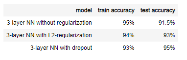
结论 三种方式的最终结果对比如下表:
我们可以学到:
正则化可以帮助减少过拟合
正则化可以迫使权重的值变得更小
L2 正则化和 dropout 正则化是两种非常有效的正则化技术
梯度检验 假设你正在搭建一个深度学习模型来检测诈骗,但是反向传播经常会有 bug,由于这是一个关键步骤,所以你的 boss 想要你的反向传播一定完全正确,所以我们在模型搭建好之后进行梯度检查。
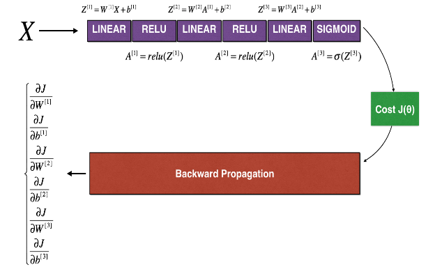
原理 反向传播计算梯度 $\frac{\partial J}{\partial \theta}$, 其中 $\theta$ 代表模型的所有参数, $J$ 是前向传播的代价函数
由于前向传播很好实现,有十足的把握是正确的,而且非常确信代价函数 $J$ 百分百正确, 所以可以用 $J$ 来检验 $\frac{\partial J}{\partial \theta}$ 的正确性。
梯度的定义式如下:
$\frac{\partial J}{\partial \theta}$ 是我们需要检验是否计算正确的梯度
我们需要计算 $J(\theta + \varepsilon)$ 和 $J(\theta - \varepsilon)$ ,因为 $J$ 是一定正确的
假设我们有个三层的模型:
先引入所需要的包:
1
2
3
import numpy as npfrom testCases import *from gc_utils import sigmoid, relu, dictionary_to_vector, vector_to_dictionary, gradients_to_vector
然后是我们已经实现好的前向传播:
1
2
3
4
5
6
7
8
9
10
11
12
13
14
15
16
17
18
19
20
21
22
23
24
25
26
27
28
29
30
31
32
33
34
35
36
37
38
39
40
41
42
43
def forward_propagation_n (X, Y, parameters) : """ Implements the forward propagation (and computes the cost) presented in Figure 3. Arguments: X -- training set for m examples Y -- labels for m examples parameters -- python dictionary containing your parameters "W1", "b1", "W2", "b2", "W3", "b3": W1 -- weight matrix of shape (5, 4) b1 -- bias vector of shape (5, 1) W2 -- weight matrix of shape (3, 5) b2 -- bias vector of shape (3, 1) W3 -- weight matrix of shape (1, 3) b3 -- bias vector of shape (1, 1) Returns: cost -- the cost function (logistic cost for one example) """ m = X.shape[1 ] W1 = parameters["W1" ] b1 = parameters["b1" ] W2 = parameters["W2" ] b2 = parameters["b2" ] W3 = parameters["W3" ] b3 = parameters["b3" ] Z1 = np.dot(W1, X) + b1 A1 = relu(Z1) Z2 = np.dot(W2, A1) + b2 A2 = relu(Z2) Z3 = np.dot(W3, A2) + b3 A3 = sigmoid(Z3) logprobs = np.multiply(-np.log(A3),Y) + np.multiply(-np.log(1 - A3), 1 - Y) cost = 1. /m * np.sum(logprobs) cache = (Z1, A1, W1, b1, Z2, A2, W2, b2, Z3, A3, W3, b3) return cost, cache
实现好的反向传播:
1
2
3
4
5
6
7
8
9
10
11
12
13
14
15
16
17
18
19
20
21
22
23
24
25
26
27
28
29
30
31
32
33
34
35
def backward_propagation_n (X, Y, cache) : """ Implement the backward propagation presented in figure 2. Arguments: X -- input datapoint, of shape (input size, 1) Y -- true "label" cache -- cache output from forward_propagation_n() Returns: gradients -- A dictionary with the gradients of the cost with respect to each parameter, activation and pre-activation variables. """ m = X.shape[1 ] (Z1, A1, W1, b1, Z2, A2, W2, b2, Z3, A3, W3, b3) = cache dZ3 = A3 - Y dW3 = 1. /m * np.dot(dZ3, A2.T) db3 = 1. /m * np.sum(dZ3, axis=1 , keepdims = True ) dA2 = np.dot(W3.T, dZ3) dZ2 = np.multiply(dA2, np.int64(A2 > 0 )) dW2 = 1. /m * np.dot(dZ2, A1.T) db2 = 1. /m * np.sum(dZ2, axis=1 , keepdims = True ) dA1 = np.dot(W2.T, dZ2) dZ1 = np.multiply(dA1, np.int64(A1 > 0 )) dW1 = 1. /m * np.dot(dZ1, X.T) db1 = 1. /m * np.sum(dZ1, axis=1 , keepdims = True ) gradients = {"dZ3" : dZ3, "dW3" : dW3, "db3" : db3, "dA2" : dA2, "dZ2" : dZ2, "dW2" : dW2, "db2" : db2, "dA1" : dA1, "dZ1" : dZ1, "dW1" : dW1, "db1" : db1} return gradients
不确定我们刚刚实现的反向传播是否正确,所以我们写一个梯度检验的函数。
多参数梯度检验的实现 对于下式:
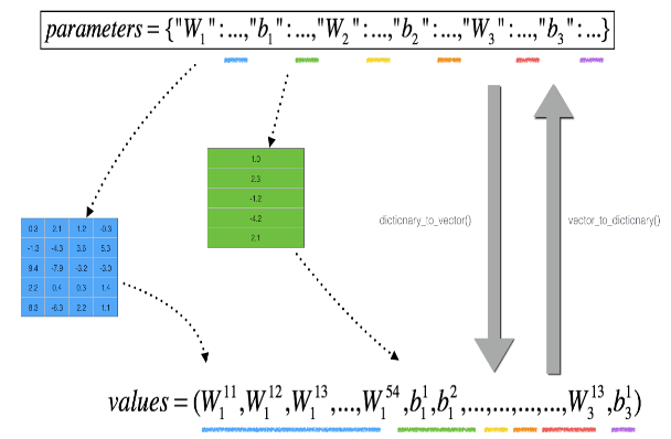
其中 $\theta$ 不是一个标量,而是一个字典 parameters,所以我们需要先将这个字典转化为一个向量 parameters_value,方便进行取值,转化的过程如下图所示:
将字典转化为向量的函数 dictionary_to_vector() 和将向量转化回字典的函数 vector_to_dictionary() 和将梯度字典转化为梯度向量的函数 gradients_to_vector() 代码如下:
1
2
3
4
5
6
7
8
9
10
11
12
13
14
15
16
17
18
19
20
21
22
23
24
25
26
27
28
29
30
31
32
33
34
35
36
37
38
39
40
41
42
43
44
45
46
47
48
49
50
51
def dictionary_to_vector (parameters) : """ Roll all our parameters dictionary into a single vector satisfying our specific required shape. """ keys = [] count = 0 for key in ["W1" , "b1" , "W2" , "b2" , "W3" , "b3" ]: new_vector = np.reshape(parameters[key], (-1 ,1 )) keys = keys + [key]*new_vector.shape[0 ] if count == 0 : theta = new_vector else : theta = np.concatenate((theta, new_vector), axis=0 ) count = count + 1 return theta, keys def vector_to_dictionary (theta) : """ Unroll all our parameters dictionary from a single vector satisfying our specific required shape. """ parameters = {} parameters["W1" ] = theta[:20 ].reshape((5 ,4 )) parameters["b1" ] = theta[20 :25 ].reshape((5 ,1 )) parameters["W2" ] = theta[25 :40 ].reshape((3 ,5 )) parameters["b2" ] = theta[40 :43 ].reshape((3 ,1 )) parameters["W3" ] = theta[43 :46 ].reshape((1 ,3 )) parameters["b3" ] = theta[46 :47 ].reshape((1 ,1 )) return parameters def gradients_to_vector (gradients) : """ Roll all our gradients dictionary into a single vector satisfying our specific required shape. """ count = 0 for key in ["dW1" , "db1" , "dW2" , "db2" , "dW3" , "db3" ]: new_vector = np.reshape(gradients[key], (-1 ,1 )) if count == 0 : theta = new_vector else : theta = np.concatenate((theta, new_vector), axis=0 ) count = count + 1 return theta
现在我们得到了 paremeters_values (也就是 $\theta$) 的向量,下面是进行梯度检查的步骤:
for each i in len(paremeters_values):
计算 $J(…,\theta[i]+\varepsilon,…)$,即 J_plus[i]:
$\theta^+$ = np.copy(parameters_values)
$\theta^+[i]=\theta^+[i]+\varepsilon$
将 $\theta^+$ 重新转换回参数字典(使用 vector_to_dictionary 函数)
用新的参数带入前向传播计算 J_plus[i]
同样的方法计算$J(…,\theta[i]-\varepsilon,…)$,即 J_minus[i]
用梯度估算式计算梯度 $gradapprox[i]=\frac{J_plus[i]-J_minus[i]}{2\varepsilon}$
计算估算值和实际值的差异:$ difference = \frac {| grad - gradapprox |_2}{| grad |_2 + | gradapprox |_2 } $
实现代码如下:
1
2
3
4
5
6
7
8
9
10
11
12
13
14
15
16
17
18
19
20
21
22
23
24
25
26
27
28
29
30
31
32
33
34
35
36
37
38
39
40
41
42
43
44
45
46
47
48
49
50
def gradient_check_n (parameters, gradients, X, Y, epsilon = 1e-7 ) : """ 检查反向传播计算的梯度是否正确 Arguments: parameters -- python dictionary containing your parameters "W1", "b1", "W2", "b2", "W3", "b3": gradients -- 反向传播的输出,包含了代价函数对 theta 中每个参数的梯度的实际计算值的字典,需要检验正确性 X -- input datapoint, of shape (input size, 1) Y -- true "label" epsilon -- tiny shift to the input to compute approximated gradient with formula(1) Returns: difference -- difference (2) between the approximated gradient and the backward propagation gradient """ parameters_values, _ = dictionary_to_vector(parameters) grad = gradients_to_vector(gradients) num_parameters = parameters_values.shape[0 ] J_plus = np.zeros((num_parameters, 1 )) J_minus = np.zeros((num_parameters, 1 )) gradapprox = np.zeros((num_parameters, 1 )) for i in range(num_parameters): thetaplus = np.copy(parameters_values) thetaplus[i][0 ] = thetaplus[i][0 ] + epsilon J_plus[i], _ =forward_propagation_n(X, Y, vector_to_dictionary(thetaplus)) thetaminus = np.copy(parameters_values) thetaminus[i][0 ] = thetaminus[i][0 ] - epsilon J_minus[i], _ = forward_propagation_n(X,Y,vector_to_dictionary(thetaminus)) gradapprox[i] = (J_plus[i]-J_minus[i]) / np.float(2 * epsilon) numerator = np.linalg.norm(grad-gradapprox) denominator = np.linalg.norm(grad) + np.linalg.norm(gradapprox) difference = numerator / denominator if difference > 1e-7 : print ("\033[93m" + "There is a mistake in the backward propagation! difference = " + str(difference) + "\033[0m" ) else : print ("\033[92m" + "Your backward propagation works perfectly fine! difference = " + str(difference) + "\033[0m" ) return difference
下面运用这个函数来对我们的反向传播进行检验:
1
2
3
4
5
X, Y, parameters = gradient_check_n_test_case() cost, cache = forward_propagation_n(X, Y, parameters) gradients = backward_propagation_n(X, Y, cache) difference = gradient_check_n(parameters, gradients, X, Y)
>> There is a mistake in the backward propagation! difference = 1.18904178788e-07
结果显示,梯度检验可能没有通过,反向传播中可能有错误,于是我们可以返回之前写的反向传播中进行仔细检查!
注意事项
由于 $\frac{\partial J}{\partial \theta} \approx \frac{J(\theta + \varepsilon) - J(\theta - \varepsilon)}{2 \varepsilon}$ 的计算成本很高,所以梯度检验非常慢,因此不要在训练的时候进行梯度检验,只需要调用几次检验反向传播函数是否正确即可
梯度检验不能与 dropout 一起运行,可以在运行梯度检验之前先关掉 dropout,检验完后再打开
总结
梯度检验核实了反向传播中计算的梯度和公式估计的梯度之间的接近程度
梯度检验很慢,所以不要在训练的每一次迭代中运行,只有当你想确保你的代码正确的时候才要用,然后在实际的学习过程中关掉它